Exercises: Gene prediction

Exercise 4.1. Open Reading Frame (ORF) determination

Step 1: Download the genomic sequence of a gene with one exon (together with a total flanking sequence, right and left, of 1 kb)

For example: ATOH gene

Hints and tricks:

• Use the Table Browser for the UCSC Genome Browser so identify a list of genes with one exon (for example: Genes and gene predictions > RefSeq genes > Refgene > Filter: ExonCount = 1 > output as hyperlinks in Genome Browser)

Download ORFs UCSC

Step 2: Use EMBOSS getorf to determine ORFs in the sequence

What are the default settings for minsize and maxsize?

getorf -sequence atoh1.fa -minsize 100 -outseq atoh1_orf.fa

Hints and tricks:

• Count the number of ORFs

  cat atoh1.fa | grep '>' | wc -l

Step 3: Use EMBOSS plotorf to plot the location of the identified ORFs in the sequence (graphtype = png)

plotorf -sequence atoh1.fa -graph png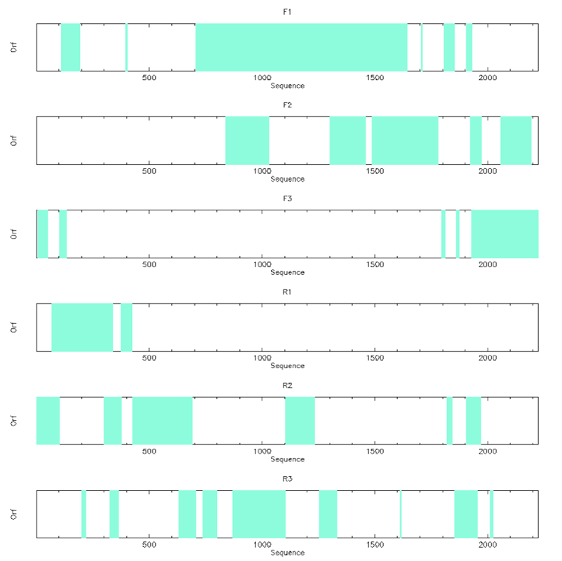

plotorf

Exercise 4.2. Coding statistics

Step 1: Use EMBOSS syco to calculate the codon usage on the sequence from exercise 4.1. (codon usage file for human: Ehum.cut)

ls -l /usr/share/EMBOSS/data/CODONS/*.cut
syco -sequence atoh1.fa -cfuke Ehum.cut -graph png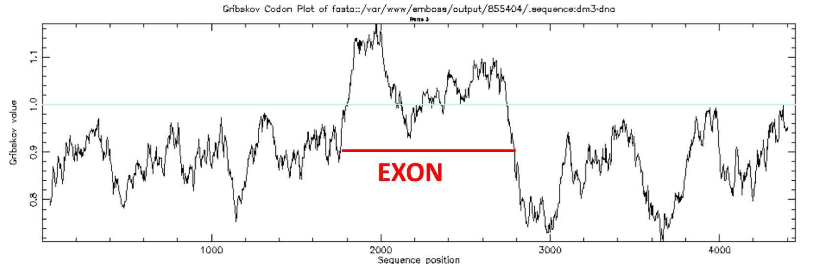

Coding statistics plot: syco

Step 2: Use tcode for a combination of codon usage with periodicity scores

tcode -sequence mySeq.fa -outfile mySeq.tcode -window 200 -plot Y -graph png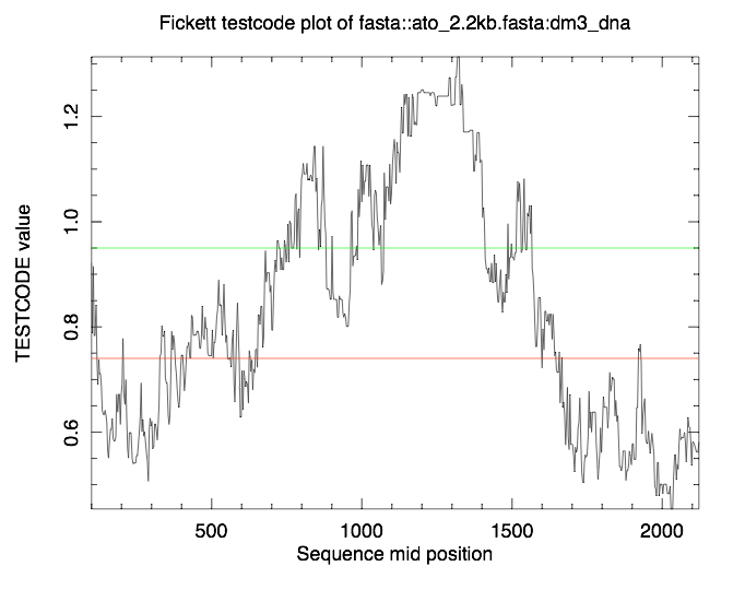

Coding statistics plot: tcode

Exercise 4.3. GeneID

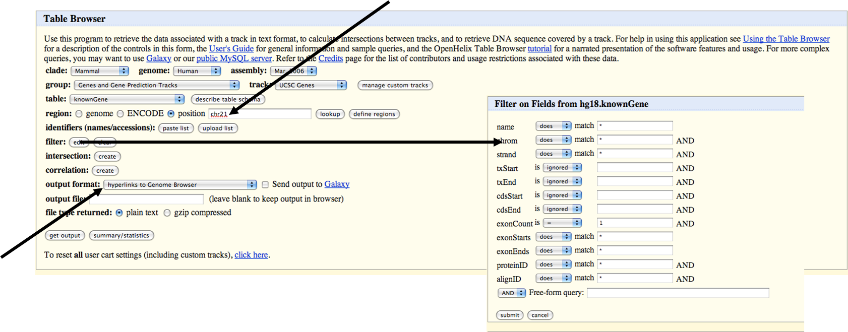
Step 1: Retrieve DNA sequence of the first Mb of human chromosome 20 (genome assembly hg18) via the command-line

Hints and tricks:

• Download chromosome 20 from the UCSC Genome Browser
• Use wget in the command-line with the above link to download files from a web site
• This file is is .gzip (.gz) file, which represents an archive file format for data compression -> unzip the file with gunzip on the command-line
• Use EMBOSS extractseq to extract the first 1 Mb of the sequence
• Chr20 file can also be found: /home/saerts/chr20/chr20.fa

Try to get the FASTA sequence for this region also using the UCSC Genome Browser, the UCSC Table Browser or the Ensembl Genome Browser.

Step 2: Predict genes with GeneID and output in GFF file format

geneid -vP human3iso.param chr20_FirstMb.fa -G > chr20_FirstMb_geneid.gff

Hints and tricks:

• A parameter file with several parameters, such as codon probability values, needs to be specified when using GeneID with -P
• Locate the parameter file with locate human3iso.param in the command-line (location: /opt/geneid/param/human3iso.param)
• Use -v to display info messages during the process of gene prediction

Step 3: Upload output GFF file as a custom track in the UCSC Genome Browser and compare with the UCSC Genes track

Hints and tricks:

• To specify you track name and color, change track settings in the UCSC Genome Browser (Manage tracks) or add the following to the first line of your GFF file (in a text editor):

  track name='GeneID' color=255,0,0 description='User Supplied Track'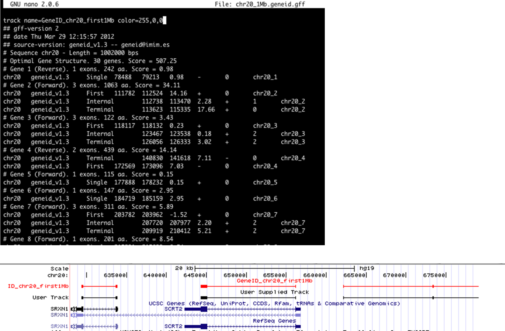

Custom track color and name in the UCSC Genome Browser

Exercise 4.4. GeneID

Use a 1 Mb sequence around the human URO-D gene to perform gene prediction (GeneID, Genscan) in this region. From the gene prediction output create a custom track file in BED or GFF format with the correct genomic coordinates (Hint: use Excel, see Hints and tricks). Visualize your file as a track in the UCSC Genome Browser and compare with UCSC Genes and RefSeq genes track.

Hints and tricks:

• Caution: be aware of genes on the negative strand!
• Do not forget to take the reverse complement if you download the sequence via the gene
• Use the UCSC Genome Browser to download DNA sequence, instead of via the gene

• For coordinate conversion the GFF output needs to be saved as a text file. Copy the GFF output into a text editor and save as text file. Open this text file with Excel.

  A text import window will pop up, continue with default settings and press Finish.

  

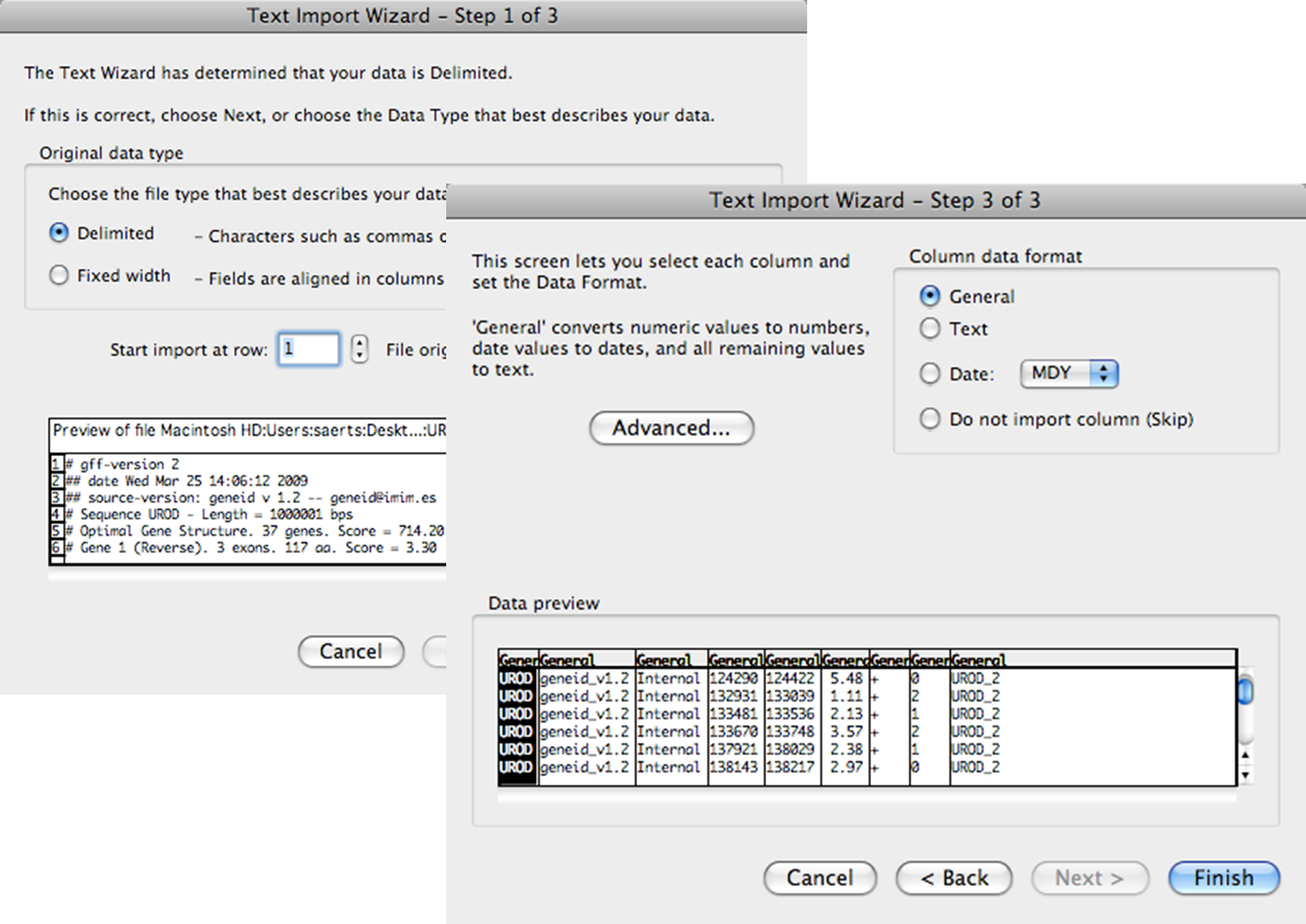
  Excel Text Import Wizard

  Remove lines with #: Select all data -> Data Sort (descending on column G (=start position)). Lines with # will be at the bottom of the file -> delete

  Add the genomic location (minus 1) to the start position in the file. Use the fill handle in Excel (Place your mouse in the lower right corner and drag down to copy)

  Add the genomic location (minus 1) to the end position in the file.

  Change the name of the chromosome (first column) into the chromosome number.

  Copy whole data table and paste in text editor (Notepad++) -> Save as GFF file

Exercise 4.5. Coordinate conversion

Coordinate conversion can also be performed through the command-line. Use the awk statement:

Define a variable with a position in the command-line for example:

offset=44750000

cat geneid_predictions.gff | awk '{ print "chr1",$2,$3,$4+offset,$5+offset,$6,$7,$8,$9}'| tr' ' '\t'     

A Python script can also be used for coordinate conversion.

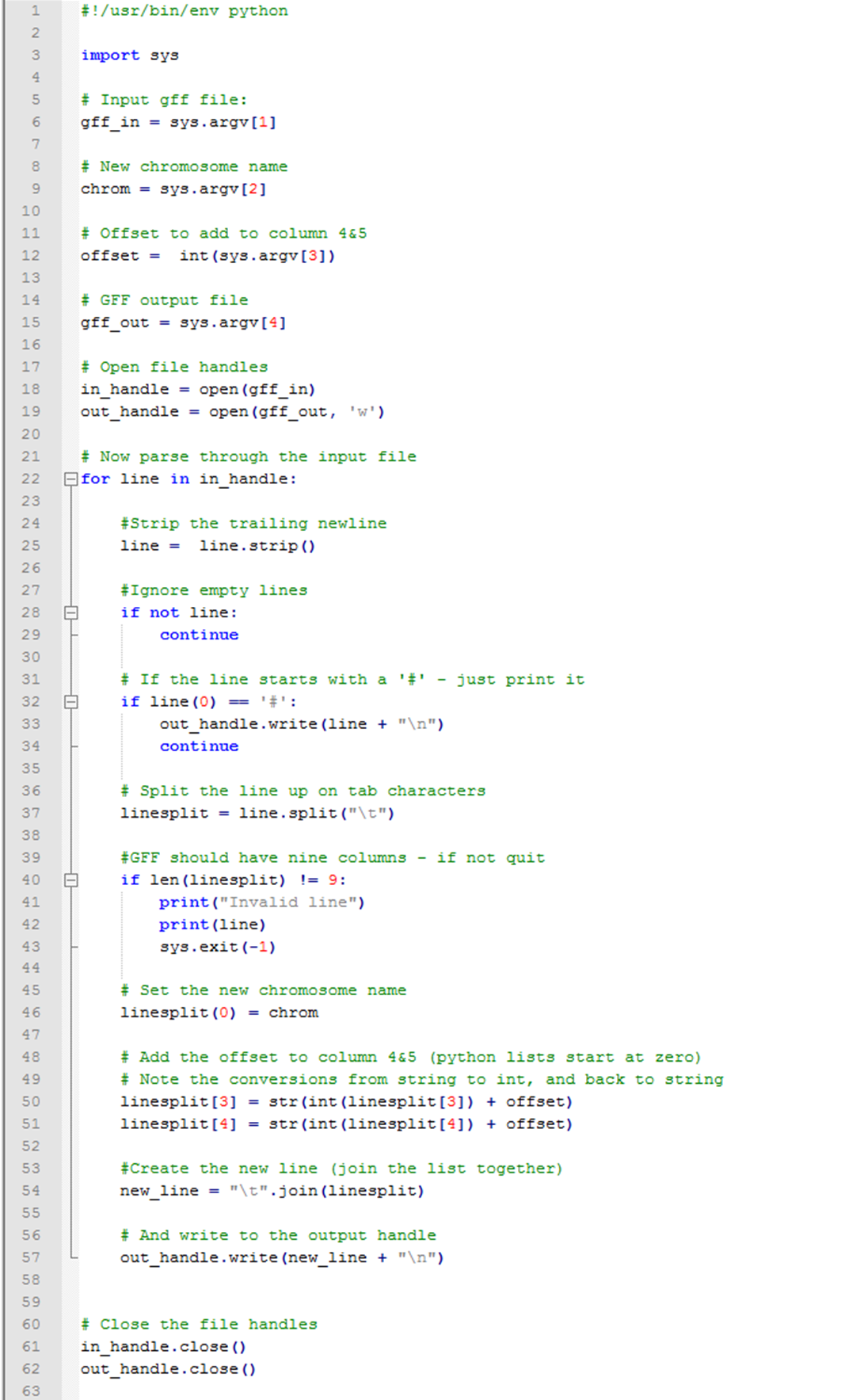
Python script for coordinate conversion

Exercise 4.6. Gene prediction accuracy

Step 1: Use the gene prediction track you have uploaded in Exercise 4.4.

Step 2: Compare your gene predictions to the UCSC Genes track by using intersections at the UCSC Table Browser (at the gene level, not at nucleotide or exon level)

How many GeneID predicted genes overlap with the UCSC Genes (i.e. How many true positives)?

How many and what kind of UCSC Genes are missed by GeneID (i.e. How many false negatives)?

How many genes are predicted by GeneID that are not UCSC Genes (i.e. How many false positives)?

Solution Exercise 4.6. Gene prediction accuracy